
While terms like Artificial Intelligence (AI), Machine Learning (ML), and Deep Learning (DL) are frequently used interchangeably in technology news, they represent distinct, nested levels of computational architecture. Machine Learning is a subset of Artificial Intelligence that enables computers to learn from data without explicit programming. Deep Learning, in turn, is a specialized subfield of Machine Learning powered by multi-layered artificial neural networks designed to mimic the human brain’s processing structure.
The primary inflection point between classical machine learning and deep learning lies in **feature engineering**. In traditional machine learning, human domain experts must manually clean, select, and extract numerical features from raw inputs before feeding them to an algorithm. Deep learning eliminates this manual bottleneck through **automated feature extraction**, allowing multi-layered neural networks to learn representations directly from raw, unstructured data such as audio, images, video, and text.
In this technical guide, we break down how deep learning operates, explore artificial neural network architectures, evaluate deep learning against classical machine learning across core technical benchmarks, and review real-world enterprise applications.
1. AI vs. Machine Learning vs. Deep Learning: The Nested Architecture
To understand where deep learning fits into the broader technology ecosystem, consider its position within the nested hierarchy of artificial intelligence.
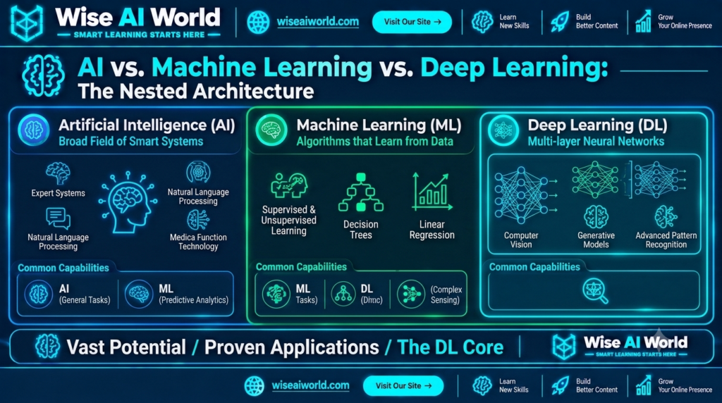
Defining the Three Layers
- Artificial Intelligence (AI): The overarching discipline focused on creating systems capable of performing tasks that typically require human intelligence, including rule-based expert systems and logic engines.
- Machine Learning (ML): A subset of AI where algorithms learn statistical relationships from structured datasets to make predictions or decisions without being explicitly programmed.
- Deep Learning (DL): A subset of ML utilizing Deep Neural Networks (DNNs) with multiple hidden layers capable of processing massive volumes of unstructured data through automatic feature hierarchy learning.
2. How Deep Learning Works: Artificial Neural Network (ANN) Anatomy
At the core of deep learning is the **Artificial Neural Network (ANN)**, inspired by biological neuronal networks in human cerebral cortexes. Information flows sequentially through distinct node layers during model processing.
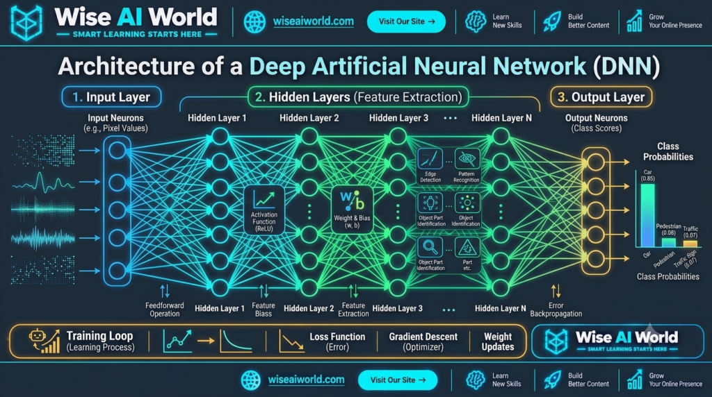
The Core Layers of a Deep Network
- Input Layer: Receives raw data vectors (e.g., individual pixel RGB values for an image or word embeddings for a text sequence).
- Hidden Layers: Intermediate node layers where mathematical transformations take place. Networks with more than three hidden layers are mathematically classified as “deep” neural networks.
- Nodes (Neurons): Computational units within layers that calculate weighted sums of inputs, apply a bias term, and pass the result through a non-linear Activation Function (such as ReLU, Sigmoid, or GELU).
- Output Layer: Produces final model predictions, such as class probability scores across target categories.
The Learning Engine: Forward & Backward Pass
Deep neural networks learn through two complementary operations:
- Forward Propagation: Input data passes sequentially through hidden layers to compute a prediction. The network calculates its error by comparing this prediction against ground-truth labels using a Loss Function (e.g., Cross-Entropy Loss or Mean Squared Error).
- Backpropagation & Gradient Descent: The calculated error propagates backward through the network. Using differential calculus (the chain rule), optimization algorithms like Adam or Stochastic Gradient Descent (SGD) update internal weights and biases to minimize future error.
3. Key Architectural Differences: Machine Learning vs. Deep Learning
Selecting between classical machine learning and deep learning depends on data scale, hardware infrastructure, and operational requirements.
| Architectural Attribute | Classical Machine Learning | Deep Learning |
|---|---|---|
| Feature Engineering | Requires manual domain-expert feature extraction. | Automated hierarchical feature learning from raw data. |
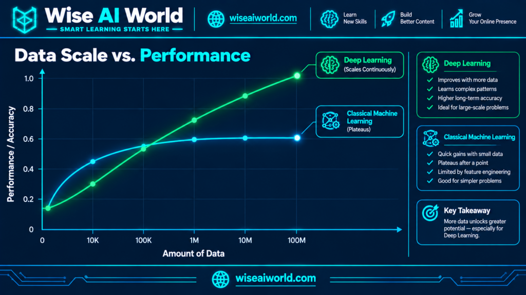
| Data Scale Performance | Performance plateaus as data volume scales beyond threshold. | Performance improves continuously with larger datasets. |
| Hardware Requirements | Runs efficiently on standard multi-core CPUs. | Requires parallel computing acceleration (NVIDIA GPUs / TPUs). |
| Training Time | Fast training (seconds to hours). | Compute-intensive training (hours to weeks). |
| Interpretability | High (Decision Trees, Linear Models offer clear feature attribution). | Low (“Black box” representation requiring SHAP/LIME inspection). |
A. The Data Scaling Curve
Classical machine learning models like Random Forests or Support Vector Machines excel on small-to-medium tabular datasets. However, their performance curve flattens once data reaches gigabyte scales. Deep learning models continue to scale accuracy as training data expands into terabyte ranges.
4. Common Deep Learning Neural Network Architectures
Different enterprise challenges require specialized deep neural network topologies engineered for specific data modalities.
- Convolutional Neural Networks (CNNs): Designed for spatial data like images and video. CNNs utilize spatial convolution kernels to scan inputs for local features like edges, textures, and object components.
- Recurrent Neural Networks (RNNs) & LSTMs: Tailored for sequential data like time-series financial metrics or audio signals. Long Short-Term Memory (LSTM) networks maintain internal memory states across time steps.
- Transformers: The dominant modern architecture for processing sequence data. Utilizing self-attention mechanisms, Transformers compute global dependencies in parallel, powering Large Language Models (LLMs) like GPT-4, Claude 3.5, and Llama 3.
5. Practical Python Implementation: Deep Learning Image Classifier with PyTorch
Below is a production-ready Python script utilizing PyTorch to define and train a simple Deep Convolutional Neural Network (CNN) for image classification.
import torch
import torch.nn as nn
import torch.optim as optim

# Step 1: Define Deep Convolutional Neural Network (CNN) Architecture
class DeepImageClassifier(nn.Module):
    def __init__(self, num_classes=10):
        super(DeepImageClassifier, self).__init__()
        # Feature Extraction Layers
        self.features = nn.Sequential(
            nn.Conv2d(in_channels=3, out_channels=32, kernel_size=3, padding=1),
            nn.BatchNorm2d(32),
            nn.ReLU(),
            nn.MaxPool2d(kernel_size=2, stride=2), # Downsample 32x32 to 16x16

            nn.Conv2d(in_channels=32, out_channels=64, kernel_size=3, padding=1),
            nn.BatchNorm2d(64),
            nn.ReLU(),
            nn.MaxPool2d(kernel_size=2, stride=2)  # Downsample 16x16 to 8x8
        )
        # Fully Connected Classification Head
        self.classifier = nn.Sequential(
            nn.Flatten(),
            nn.Linear(64 * 8 * 8, 128),
            nn.ReLU(),
            nn.Dropout(0.5),
            nn.Linear(128, num_classes)
        )

    def forward(self, x):
        x = self.features(x)
        x = self.classifier(x)
        return x

# Step 2: Initialize Model, Loss Function, and Optimizer
device = torch.device("cuda" if torch.cuda.is_available() else "cpu")
model = DeepImageClassifier(num_classes=10).to(device)

criterion = nn.CrossEntropyLoss()
optimizer = optim.Adam(model.parameters(), lr=0.001)

print(f"Deep Learning Model Initialized on Device: {device}")
print(f"Total Model Parameters: {sum(p.numel() for p in model.parameters()):,}")

# Step 3: Synthetic Forward Pass Simulation (Batch of 4 RGB Images, 32x32 pixels)
dummy_batch = torch.randn(4, 3, 32, 32).to(device)
output_logits = model(dummy_batch)
print(f"Output Batch Predictions Shape: {output_logits.shape}")
6. Summary & Decision Matrix
Understanding when to deploy classical machine learning versus deep learning is an essential architecture decision for technical leaders.
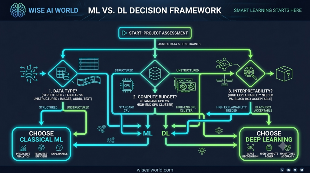
Quick Decision Framework:
- Choose Classical Machine Learning if: Your dataset is structured/tabular (CSVs, SQL tables), dataset size is under 100,000 rows, CPU hardware is constrained, or strict regulatory explainability is required.
- Choose Deep Learning if: Your dataset consists of unstructured media (text, images, audio, video), data volume is vast, GPU acceleration is available, and maximizing raw predictive accuracy is the primary goal.
Disclosure: WiseAIWorld independently tests and benchmarks AI frameworks and computing platforms. Some links on this site contain affiliate tracking links. If you sign up through our links, we may receive a small commission at no additional cost to you.

Manish Prakash Dubey is an AI educator and technology writer based in India. He founded WiseAIWorld to make artificial intelligence simple and practical for students, professionals, and beginners. His work focuses on AI basics, machine learning, deep learning, NLP, computer vision, and real-world AI tools.
